
A bit more good news about polar bear populations, this time from an abundance study in the Southern Beaufort Sea. A paper released yesterday showed a 25-50% decline in population size took place between 2004 and 2006 (larger than previously calculated). However, by 2010 the population had rebounded substantially (although not to previous levels).
All the media headlines (e.g. The Guardian) have followed the press release lead and focused on the extent of the decline. However, it’s the recovery portion of the study that’s the real news, as it’s based on new data. Such a recovery is similar to one documented in the late 1970s after a significant decline occurred in 1974-1976 that was caused by thick spring ice conditions.

The title of the new paper by Jeffery Bromaghin and a string of polar bear biologists and modeling specialists (including all the big guns: Stirling, Derocher, Regehr, and Amstrup) is “Polar bear population dynamics in the southern Beaufort Sea during a period of sea ice decline.” However, the study did not find any correlation of population decline with ice conditions. They did not find any correlation with ice conditions because they did not include spring ice thickness in their models – they only considered summer ice conditions.
I find this very odd, since previous instances of this phenomenon, which have occurred every 10 years or so since the 1960s, have all been associated with thick spring ice conditions (the 1974-76 and 2004-2006 events were the worst). [Another incident may have occurred this spring (April 2014) but has not been confirmed].
Whoever wrote the press release for this paper tried hard to suggest the cause of the 2004-2006 event might have been “thin” winter ice caused by global warming that was later deformed into thick spring ice, an absurd excuse that has been tried before (discussed here). If so, what caused the 1974-1976 event?
It seems rather unscientific as well as implausible to even try to blame this recent phenomenon on global warming. However, neither the authors of the paper or the press release writers seemed to want to admit that 2-3 years of thick ice development in the Southern Beaufort could have been the cause of the population decline in 2004 (as for all of the previous events). No, that wouldn’t do, not in the age of global warming.
So, we are left with this equally absurd conclusion from the author:
“The low survival may have been caused by a combination of factors that could be difficult to unravel,” said Bromaghin, “and why survival improved at the end of the study is unknown.”
I’ve summarized the paper to the best of my understanding (there was a lot of model-speak to wade through), leaving out the prophesies of extinction, which in my opinion don’t add anything.
UPDATE November 19, 2014: Don’t miss my follow-up post, with some startling new information, “Polar bear researchers knew S. Beaufort population continued to increase up to 2012“
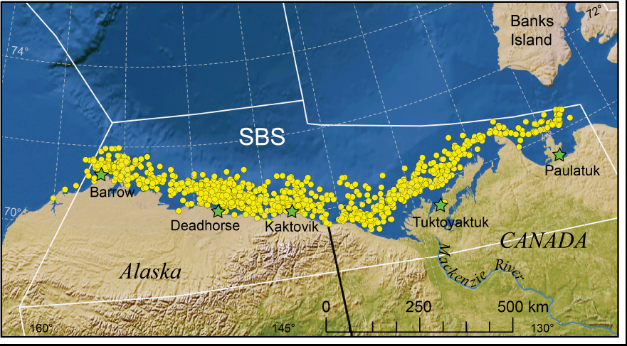
Figure 1. This is Fig. 1 from Bromaghin et al. 2015 2014 in press, showing the study area. Note about half of the Southern Beaufort Sea subpopulation is in the USA and the other half is in Canada. Canada has recently moved the eastern boundary to ~ Tuktoyaktuk.
Summary of results:
“Our results collectively suggest that polar bears in the SBS experienced a significant reduction in survival and abundance from 2004 through 2007. However, suspected biases in the abundance estimates for the earliest years of the investigation, potential biases in the USCA estimates in the latter years, and statistical variation associated with estimates necessitate cautious expression of the magnitude of population decline. Conservatively, the decline seems unlikely to have been less than 25%, but may have approached 50%. Improved survival and stability in abundance at the end of the investigation are cause for cautious optimism.”
…
Extensive ice rubble and rafted floes during winter and spring are thought to have led to past declines in polar bear productivity in the SBS (Stirling et al. 1976, Amstrup et al. 1986, Stirling 2002), as well as during our investigation (Stirling et al. 2008). [discussed here and here]
…
Despite the known importance of sea ice, measures of ice availability did not fully explain short-term demographic patterns in our data, suggesting that other aspects of the ecosystem contribute importantly to the regulation of population dynamics.
…
For reasons that are not clear, survival of adults and cubs began to improve in 2007 and abundance was comparatively stable from 2008 to 2010 with approximately 900 bears in 2010 (90% C.I. 606-1,212). However, survival of subadult bears declined throughout the entire period.
…
However, in the short term, our findings suggest that factors other than sea ice can influence survival.” [my bold]
Note that summer sea ice was the only ice condition they examined. And note that the second-lowest September sea ice minimum, which occurred in 2007, was the point at which survival of adults and cubs began to improve.
![Figure 2. Bromaghin et al. 2014 in press, FIG. 5. Model-averaged estimates of abundance based on (a) the USGS data set [USA half of SBS only] and (b) the USCA data set [Canadian half of SBS only]. Error bars represent 90% bias-corrected confidence intervals based on 100 bootstrap samples. Prior estimates (Regehr et al. 2006) are shown for comparative purposes (b, open diamonds). This reminds me of the 2011 Northern Beaufort Sea population estimate graph discussed here, about which eminent ecologist Dr. Daniel Botkin remarked: “The confidence intervals are so large that nothing can be concluded.”](https://polarbearscience.com/wp-content/uploads/2014/11/bromighan-et-al-2014-in-press-fig-5-abundance.jpg)
Figure 2. Bromaghin et al. 2015 2014 in press, FIG. 5. “Model-averaged estimates of abundance based on (a) the USGS data set [USA half of SBS only] and (b) the USCA data set [Canadian half of SBS only]. Error bars represent 90% bias-corrected confidence intervals based on 100 bootstrap samples. Prior estimates (Regehr et al. 2006) are shown for comparative purposes (b, open diamonds).” [SJC: This graph reminds me of the 2011 Northern Beaufort Sea population estimate graph discussed here, about which eminent ecologist Dr. Daniel Botkin remarked: “The confidence intervals are so large that nothing can be concluded.” ]
As far as I can tell, Bromaghin et al. 2015 2014 appears to be a re-analysis of Regehr et al.’s (2006) data with a few more years added. Oddly, Regehr et al. 2006 found a statistically insignificant decline from 2001 to 2006 while the re-analysis by Bromaghin et al. (2015 2014), using a new and improved method developed by Bromaghin et al. (2013), found a substantial decline and only a moderate recovery between 2001-2010.
Are the large decline and modest recovery real — more real than previous estimates? In my opinion, it will take a very long and careful examination by modeling experts to determine that answer. Contact me if you would like a copy of the paper. Final, in-print version of the paper is open access. More details below on the methods.
![Figure 3. Bromaghin et al. 2014 in press, FIG. 2. Anomalies (difference from the mean) of the two sea ice covariates from 1979 to 2010. Normalized values from 2001 to 2010 (dark grey) were used to model polar bear survival probabilities; (a) Summer-habitat, and (b) Melt-season. [“Summer-habitat” is area of optimal polar bear habitat, July-October; “Melt-season” is the time between melt and refreeze each summer]. The study found no correlation between population size and sea ice coverage.](https://polarbearscience.com/wp-content/uploads/2014/11/bromighan-et-al-2014-in-press-fig-2.jpg)
Figure 3. Bromaghin et al. 2015 2014 in press, FIG. 2. “Anomalies (difference from the mean) of the two sea ice covariates from 1979 to 2010. Normalized values from 2001 to 2010 (dark grey) were used to model polar bear survival probabilities; (a) Summer-habitat, and (b) Melt-season.” [SJC: “Summer-habitat” is area of optimal polar bear habitat, July-October; “Melt-season” is the time between melt and refreeze each summer. The study found no correlation between population size and sea ice coverage.]
Abundance Results
“Annual abundance estimates based on the USGS data, applicable to the Alaskan portion of the study area, ranged from 376 in 2009 to 1,158 in 2004 (Fig. 5a). We suspect estimates in the first two years, particularly 2002, were negatively biased by the absence of capture effort from Barrow in 2001, which may have caused an over-estimate of recapture probability in 2002 (Appendix C, Fig. C1-C3).
In addition, the mixing of marked and unmarked individuals may have been incomplete during the initial years of the study (Appendix D, Fig. D2). The unusually large number of bears captured in 2004 (Table 5) produced a seemingly large estimate with a wide confidence interval.
Even though there is uncertainty regarding abundance levels in these years, the broader pattern of a decline in abundance during the middle of the study followed by relative stability at the end of the study was consistent with patterns in survival.
Abundance estimates based on the USCA data ranged from 464 in 2002 to 1,607 in 2004 (Fig. 5b). As with the USGS data, we suspect estimates for the initial years of the investigation were less reliable than those in the latter years, particularly because no capture effort occurred in Canada before 2003 and our models were not robust to this deficiency.
Considering this uncertainty in the earliest estimates, the temporal pattern in abundance resembled that of the USGS estimates and was consistent with patterns in survival. The correlation between USGS and USCA abundance estimates was 0.84 across all years and 0.86 excluding 2002.” [my bold, sentence spacing added for readability]
Period of the study: 2001-2010 (2001-2005 used previously in 2008 ESA assessment).
Season of capture: Approximately late March to early May each year (April/May in Canada). Apparently, the condition of bears in summer and fall was not considered.
Method of capture: Bears were chased with helicopter, sedated, tattooed, ear tags attached; some adult females fitted with satellite radio collars in all years except 2010.
Sea ice relationships: They used only “summer-habitat” (area of optimal polar bear habitat available for July through October) and “Melt-season” (the time between melt and refreeze in the Beaufort each summer).
Areas of capture: US half (called “USGS”), 2001-2010 (late March-May); Canadian half (called “USCA”), 2003-2006 (April and May) and 2007-2010 but not to the eastern boundary (with subadults and females preferentially targeted).
Therefore, the sampling effort was uneven: there were no captures in the Canadian half of SBS from 2001and 2002 and captures were biased towards females and subadults in 2007 through 2010. But it appears to be the Canadian (“USCA”) population estimate for 2010 that is being accepted as representative. Go figure.
Method of abundance estimate: They used “open-population Cormack-Jolly-Seber (CJS) models” developed by Lebreton et al. (1992), same as used by Regehr et al. 2007, 2010 (for SBS) and Stirling et al. 2011 (for NBS). Harvested animals were accounted for, they said. Survival probabilities used by the model were calculated for cubs, yearlings, subadults and adults.
Method of evaluating models: They used a new “improved method” of evaluating the models described above, which involved computer simulation (Bromaghin et al. 2013, an open access paper listed below).
Known movement of bears between SBS, Chuckchi Sea and NBS: This is called “heterogeneity in recapture probabilities”; the authors claim they accounted for this phenomenon (which the Polar Bear Specialist Group identified as a serious problematic issue for this region, and which was not taken into account as it should have been in the last population estimate, discussed previously here) in their abundance estimates. They said:
“In summary, although we are aware of the potential influence of temporary emigration and non-random movement, we believe any bias from these sources is likely to be small compared to the magnitude of temporal variation and trends in survival and abundance estimates.”
[See also Guest post: How ‘science’ counts bears July 3, 2013]
References
Bromaghin, J.F., McDonald, T.L. and Amstrup, S.C. 2013. Plausible combinations: An improved method to evaluate the covariate structure of Cormack-Jolly-Seber mark-recapture models. Open Journal of Ecology 3:11-22 doi: 10.4236/oje.2013.31002 open access, pdf here.
From the abstract:
“We present a new strategy for searching the space of a candidate set of Cormack-Jolly-Seber models and explore its performance relative to existing strategies using computer simulation. The new strategy provides an improved assessment of the importance of covariates and covariate combinations used to model survival and recapture probabilities, while requiring only a modest increase in the number of models on which inference is based in comparison to existing techniques.”
Bromaghin, J.F., McDonald, T.L., Stirling, I., Derocher, A.E., Richardson, E.S., Rehehr, E.V., Douglas, D.C., Durner, G.M., Atwood, T. and Amstrup, S.C. 2015. 2014 in press. Polar bear population dynamics in the southern Beaufort Sea during a period of sea ice decline. Ecological Applications 25(3):634-651. http://www.esajournals.org/doi/abs/10.1890/14-1129.1 Open access.
Regehr, E.V., Amstrup, S.C., and Stirling, I. 2006. Polar bear population status in the Southern Beaufort Sea. US Geological Survey Open-File Report 2006-1337. Pdf here.
Regehr, E.V., Lunn, N.J., Amstrup, S.C., and Stirling, I. 2007. Effects of earlier sea ice breakup on survival and population size of polar bears in western Hudson Bay. Journal of Wildlife Management 71:2673-2683.
Stirling, I. 2002. Polar bears and seals in the eastern Beaufort Sea and Amundsen Gulf: a synthesis of population trends and ecological relationships over three decades. Arctic 55 (Suppl. 1):59-76. http://arctic.synergiesprairies.ca/arctic/index.php/arctic/issue/view/42
Stirling, I. and Lunn, N.J. 1997. Environmental fluctuations in arctic marine ecosystems as reflected by variability in reproduction of polar bears and ringed seals. In Ecology of Arctic Environments, Woodin, S.J. and Marquiss, M. (eds), pg. 167-181. Blackwell Science, UK.
Stirling, I., McDonald, T.L., Richardson, E.S., Regehr, E.V., and Amstrup, S.C. 2011. Polar bear population status in the northern Beaufort Sea, Canada, 1971-2006. Ecological Applications 21:859-876. http://www.esajournals.org/doi/abs/10.1890/10-0849.1
Stirling, I., Richardson, E., Thiemann, G.W. and Derocher, A.E. 2008. Unusual predation attempts of polar bears on ringed seals in the southern Beaufort Sea: possible significance of changing spring ice conditions. Arctic 61:14-22. http://arctic.synergiesprairies.ca/arctic/index.php/arctic/article/view/3/3
Stirling, I., Schweinsburg, R.E., Kolenasky, G.B., Juniper, I., Robertson, R.J., and Luttich, S. 1980. Proceedings of the 7th meeting of the Polar Bear Specialists Group IUCN/SSC, 30 January-1 February, 1979, Copenhagen, Denmark. Gland, Switzerland and Cambridge UK, IUCN., pg. 45-53.http://pbsg.npolar.no/en/meetings/ pdf of except here.


You must be logged in to post a comment.